Langevin Dynamics

Why This Matters

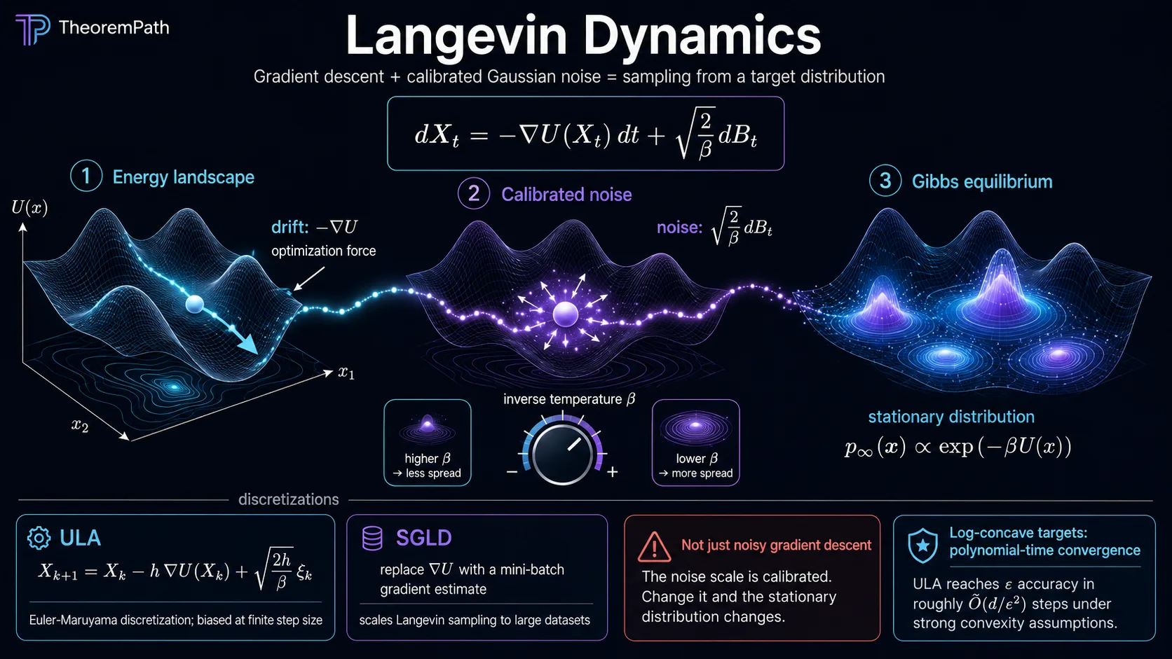
If you want to sample from a target distribution $p_\infty(x) \propto \exp(-U(x))$ and you can compute $\nabla U$, you have a clean recipe: run the SDE

$$dX_t = -\nabla U(X_t)\,dt + \sqrt{2/\beta}\,dB_t,$$

and at large $t$ the law of $X_t$ converges to $p_\infty(x) \propto \exp(-\beta U(x))$. This is overdamped Langevin dynamics. It is gradient descent on $U$ plus a precisely calibrated Gaussian noise, and the calibration is what makes the distribution — not just the trajectory — converge to the right place.

Almost every gradient-based MCMC sampler in modern ML is a discretization or perturbation of this SDE. The unadjusted Langevin algorithm (ULA) is the Euler–Maruyama discretization. SGLD (Welling–Teh 2011) replaces $\nabla U$ with a stochastic mini-batch estimate. Score-based diffusion models generate samples by running a Langevin-like reverse SDE whose drift is the learned score $\nabla \log p$. MALA, HMC, and proximal Langevin are all targeted refinements of the same machinery.

Langevin dynamics is also the SDE that gives the cleanest non-asymptotic guarantees in modern sampling theory. Dalalyan (2017) and Durmus–Moulines (2017) showed that ULA on a strongly-log-concave target reaches a prescribed total-variation distance $\varepsilon$ from $p_\infty$ in $\tilde{O}(d / \varepsilon^2)$ steps — polynomial in dimension, no intractable constants. This is the kind of guarantee Metropolis–Hastings methods cannot provide and that explains why Langevin-based methods are the default for sampling from energy-based models in dimensions above ~50.

Mental Model

Read the dynamics as a competition between two forces. The drift $-\nabla U$ pulls the particle downhill toward modes of $p_\infty$, exactly like gradient descent. The noise $\sqrt{2/\beta}\,dB$ pushes the particle around with a magnitude that scales with the inverse temperature $\beta$. At temperature $\beta = \infty$ (no noise) you recover deterministic gradient flow, which gets stuck at the nearest local minimum. At temperature $\beta = 0$ (only noise) you get pure Brownian motion, which never localizes anywhere. The Gibbs measure $\propto e^{-\beta U}$ is the unique stationary balance: probability concentrates near minima of $U$ but spreads out according to the temperature, and the relative weights between minima depend on $\beta$ times the energy gap.

The key calibration is the factor $\sqrt{2/\beta}$ in front of $dB$: any other coefficient gives a different stationary distribution. This is not a tunable hyperparameter; it is set by the requirement that the Fokker–Planck equation have $e^{-\beta U}$ as its stationary density.

Formal Definition

Definition

Overdamped Langevin SDE

For a potential $U: \mathbb{R}^d \to \mathbb{R}$ with $e^{-\beta U}$ integrable and a standard $d$-dimensional Brownian motion $B_t$, the overdamped Langevin SDE at inverse temperature $\beta$ is

$$dX_t = -\nabla U(X_t)\,dt + \sqrt{2/\beta}\,dB_t.$$

The associated Fokker–Planck equation is $\partial_t p = \nabla \cdot (\nabla U\, p) + \beta^{-1} \Delta p$, which can be rewritten in gradient-flow form $\partial_t p = \nabla \cdot \big(p\, \nabla \log(p / p_\infty)\big) / \beta$ where $p_\infty(x) = e^{-\beta U(x)}/Z$. This is the formal sense in which Langevin dynamics is the gradient flow of relative entropy $\operatorname{KL}(p \| p_\infty)$ in the Wasserstein-2 metric (Jordan, Kinderlehrer, and Otto, 1998).

The "overdamped" qualifier distinguishes this from the second-order underdamped Langevin SDE that includes a momentum variable and is the basis of Hamiltonian Monte Carlo.

Stationary Distribution

Theorem

Gibbs Measure is the Stationary Distribution of Langevin

Statement

Under the assumptions above, $p_\infty(x) = e^{-\beta U(x)}/Z$ with $Z = \int e^{-\beta U(x)}\,dx$ is the unique invariant density of the Langevin Fokker–Planck operator $\mathcal{L}^* p = \nabla \cdot (\nabla U\, p) + \beta^{-1} \Delta p$. The dynamics is reversible with respect to $p_\infty$, and detailed balance holds: the equilibrium probability current $J = -p_\infty \nabla U - \beta^{-1} \nabla p_\infty$ is identically zero.

Intuition

Plug $p_\infty$ into $\mathcal{L}^*$ and watch the cancellation. The drift term $\nabla \cdot (\nabla U\, p_\infty) = (\Delta U) p_\infty - \beta\, \lvert \nabla U \rvert^2 p_\infty$. The diffusion term $\beta^{-1} \Delta p_\infty = -\beta^{-1}(\beta\, \Delta U) p_\infty + \beta^{-1}\beta^2\, \lvert \nabla U \rvert^2 p_\infty$. They sum to zero. The factor $\sqrt{2/ \beta}$ in the SDE is exactly what makes this cancellation work.

Proof Sketch

For uniqueness, restrict to $L^2(p_\infty)$. The Fokker–Planck operator, when symmetrized as $\mathcal{L}^* = \nabla \cdot (p_\infty \nabla (\cdot / p_\infty)) / \beta$, is self-adjoint and negative semidefinite with $0$ a simple eigenvalue when $U$ has connected sublevel sets. The eigenvector for $0$ is $p_\infty$. Standard semigroup theory then gives $p(\cdot, t) \to p_\infty$ in $L^2(p_\infty)$ for any initial $p_0$ with finite relative entropy.

Why It Matters

This is the entire reason Langevin dynamics works as a sampler: with the right calibration, the SDE has the target distribution as its unique equilibrium. Tampering with the noise scale (e.g., using $\sqrt{1/\beta}$ instead of $\sqrt{2/\beta}$) changes the stationary distribution to $\propto e^{-2\beta U}$, the same modes but a sharper temperature. Methods that "anneal $\beta$" (simulated annealing) exploit this dependence to escape local minima at high temperature, then localize at low temperature. The Gibbs measure $p_\infty(x) = e^{-\beta U(x)}/Z$ is the unique stationary distribution of the overdamped Langevin SDE.

Failure Mode

The result requires $e^{-\beta U}$ to be integrable. For $U(x) = c\, x$ (linear potential) this fails: the dynamics drifts to infinity and has no stationary distribution. Same for $U$ with super-quadratic decay at infinity in some directions. Practical samplers handle this with confinement: add a quadratic regularizer $\lambda \lVert x \rVert^2 / 2$ to $U$ if the target is not provably tight.

Convergence Rate: Log-Sobolev and Bakry–Émery

The asymptotic statement "$X_t$ converges to $p_\infty$" is qualitative. The quantitative statement requires a functional inequality for the stationary measure. The cleanest one is the log-Sobolev inequality (LSI) $\operatorname{Ent}_{p_\infty}(f^2) \le \frac{2}{\rho_{\text{LSI}}}\, \mathbb{E}_{p_\infty}[\lVert \nabla f \rVert^2]$. Whenever $p_\infty$ satisfies LSI with constant $\rho_{\text{LSI}}$, the law of $X_t$ converges to $p_\infty$ in KL divergence at exponential rate $\rho_{\text{LSI}} / \beta$:

$$\operatorname{KL}\big(p(\cdot, t)\, \|\, p_\infty\big) \le e^{-2 \rho_{\text{LSI}} t / \beta}\, \operatorname{KL}\big(p_0\, \|\, p_\infty\big).$$

Bakry–Émery's curvature criterion says: if $\nabla^2 (\beta U) \succeq m\, I$ for some $m > 0$ (i.e., the rescaled potential is strongly convex), then $p_\infty$ satisfies LSI with constant at least $m$, and the convergence rate is at least $m / \beta$. This is the sharpest and cleanest convergence theorem for Langevin dynamics on log-concave targets.

For non-log-concave $p_\infty$ (multimodal energy landscapes), LSI can fail catastrophically. Holley–Stroock perturbation gives an LSI constant that scales like $e^{-\beta\, \Delta U}$ where $\Delta U$ is the energy barrier between modes, producing exponential slowdown in the barrier height. This is the mathematical statement of "Langevin gets stuck at low temperature."

Numerical Discretization: ULA

The Unadjusted Langevin Algorithm is Euler–Maruyama applied to the Langevin SDE:

$$X_{k+1} = X_k - h\, \nabla U(X_k) + \sqrt{2 h / \beta}\,\xi_k, \qquad \xi_k \stackrel{\text{iid}}{\sim} \mathcal{N}(0, I_d).$$

ULA does not exactly preserve the Gibbs measure. The discretization introduces a bias of size $O(h)$ in total variation. There is a clean non-asymptotic theory.

Theorem

Dalalyan's Non-Asymptotic ULA Bound

Statement

Under the assumptions above, the law $\mu_K^{\text{ULA}}$ of $X_K$ satisfies $\operatorname{TV}(\mu_K^{\text{ULA}}, p_\infty) \le \varepsilon$ provided $K \ge C\, \frac{d}{m\, \varepsilon^2}\, \log\!\big(\frac{1}{\varepsilon}\big)$ for an absolute constant $C$ and step size $h$ tuned proportionally to $\varepsilon^2 / d$.

Intuition

The proof couples the continuous-time Langevin SDE (which converges exponentially fast by Bakry–Émery) with its Euler–Maruyama discretization. The discretization bias accumulates linearly in the number of steps but is $O(h)$ per step, so total bias is $O(K h)$. Choosing $h$ small enough balances continuous-time convergence error against discretization bias.

Proof Sketch

Let $\mu_K^{\text{cont}}$ be the law of the continuous Langevin SDE at time $K h$. Triangle inequality: $\operatorname{TV}(\mu_K^{\text{ULA}}, p_\infty) \le \operatorname{TV}(\mu_K^{\text{ULA}}, \mu_K^{\text{cont}}) + \operatorname{TV}(\mu_K^{\text{cont}}, p_\infty)$. The first term is the discretization bias bounded via Girsanov's theorem and the Lipschitz hypothesis on $\nabla U$; it scales as $\sqrt{K h^3 d L^2}$ (Dalalyan 2017, Theorem 1). The second term decays as $e^{-m K h}$ by Bakry–Émery. Optimize $h$ over the sum.

Why It Matters

This was the first dimension-polynomial sampling result for a gradient-based MCMC method on log-concave targets. Earlier methods (MH, HMC) only had asymptotic guarantees with constants that were either intractable or known to scale exponentially in $d$. The result lit a research program: faster Langevin variants (MALA: $O(d/\varepsilon)$ gradient queries; underdamped Langevin: $\tilde{O}(\sqrt{d}/\varepsilon)$; proximal Langevin for non-smooth $U$), all measured against this baseline. After $K = O((d/m) \cdot \log(1/\varepsilon) / \varepsilon^2)$ steps, the ULA iterate is within total-variation distance $\varepsilon$ of the Gibbs measure.

Failure Mode

The result requires strong log-concavity (positive lower bound on the Hessian). Weakly log-concave or multimodal targets fall outside the hypothesis, and ULA's bias does not vanish in the standard sense. For non-log-concave problems, the Metropolis adjustment (MALA) is needed to remove the bias, but MALA's mixing time can be exponentially worse in the energy-barrier height.

Stochastic-Gradient Variant: SGLD

Welling and Teh (2011) introduced Stochastic Gradient Langevin Dynamics (SGLD): replace the exact gradient $\nabla U(X_k)$ in ULA with a mini-batch estimate $\hat{\nabla} U(X_k)$ from a random subset of data, and decay the step size $h_k \to 0$ so that the discretization bias and gradient-noise bias both vanish in the limit:

$$X_{k+1} = X_k - h_k\, \hat{\nabla} U(X_k) + \sqrt{2 h_k / \beta}\,\xi_k.$$

The intuition: at large $k$, the injected Gaussian noise $\sqrt{2 h_k / \beta}\,\xi_k$ dominates the mini-batch noise $h_k \cdot \text{stoch.\ noise}$ (because $\sqrt{h_k} \gg h_k$), and the algorithm transitions from SGD-like exploration to Langevin-like sampling. Without the decay, the mini-batch noise dominates indefinitely and the stationary distribution is not the Gibbs measure but a perturbation depending on the gradient covariance, a phenomenon that motivates the entire SGD-as-SDE literature.

Common Confusions

Watch Out

Langevin dynamics is not gradient flow

Gradient flow $\dot{x} = -\nabla U(x)$ converges to the minimizer of $U$; Langevin dynamics converges to the Gibbs distribution $\propto e^{-\beta U}$. These give different answers when $U$ is multimodal, when $\beta$ is finite, or when you care about uncertainty rather than a point estimate. The noise term is not "regularization" or "exploration heuristic" — it is what makes Langevin a sampler instead of an optimizer, and removing it loses the entire Bayesian / sampling story.

Watch Out

The step size of ULA controls bias, not variance

Standard SGD intuition: small step sizes give low variance and slow convergence, large step sizes give the opposite. For ULA the trade-off is qualitatively different: small step sizes give low bias against the true Gibbs measure but slow continuous-time mixing; large step sizes give high bias (the iterates' stationary distribution is a perturbation of Gibbs). Throwing CPU at smaller and smaller $h$ is the right move when bias is the bottleneck; there is no diminishing return on step-size shrinkage that mirrors the variance / step-size trade-off in optimization.

Watch Out

Underdamped Langevin is a different SDE, not just a numerical trick

Overdamped Langevin lives in state space $\mathbb{R}^d$. Underdamped Langevin lives in phase space $\mathbb{R}^{2d}$ with a momentum variable $V_t$ and friction coefficient $\gamma$: $dX_t = V_t\,dt$, $dV_t = -\nabla U(X_t)\,dt - \gamma V_t\,dt + \sqrt{2 \gamma / \beta}\,dB_t$. The stationary distribution is $\propto e^{-\beta (U + \lvert v \rvert^2 / 2)}$, which marginalizes back to Gibbs in $x$. The mixing time scales as $\sqrt{d}$ instead of $d$ because momentum gives the dynamics inertia to traverse low-curvature regions faster. This is the SDE behind HMC.

Exercises

ExerciseCore

Problem

For the Gaussian target $p_\infty \propto e^{-\beta x^2 / 2}$ on $\mathbb{R}$, write out the Langevin SDE explicitly, solve it in closed form starting from $X_0 = x_0$, and compute the variance of $X_t$. Confirm that $\operatorname{Var}(X_t) \to 1/\beta$ as $t \to \infty$, matching the Gibbs marginal.

Hint

Reveal Solution

ExerciseAdvanced

Problem

Consider a "double-well" potential $U(x) = (x^2 - 1)^2 / 4$ on $\mathbb{R}$. Show that the LSI constant of the Gibbs measure $p_\infty \propto e^{-\beta U}$ degrades exponentially in $\beta$ as $\beta \to \infty$, and explain what this implies for the mixing time of Langevin dynamics on this target.

Hint

Reveal Solution

References

Next Topics

• Score Matching: training a network on $\nabla \log p$, the same vector field that drives Langevin dynamics when $p = p_\infty$.
• SGD as SDE: SGD viewed as a Langevin-like SDE where the gradient noise plays the role of $\sqrt{2/\beta}\,dB$.
• Diffusion Models: generative models that sample by running a reverse Langevin-style SDE with learned drift.
• Time Reversal of SDEs: the SDE-reversal result that turns forward Langevin noising into a backward sampler.
• Stochastic Differential Equations: the parent framework Langevin specializes.

References

Canonical:
- Pavliotis, Stochastic Processes and Applications (Springer, 2014), Chapter 4. Cleanest modern treatment, including ergodicity, spectral gap, and exit-time theory for Langevin.
- Bakry, Gentil, and Ledoux, Analysis and Geometry of Markov Diffusion Operators (Springer Grundlehren, 2014). The authoritative reference on log-Sobolev, Bakry-Emery curvature, and exponential ergodicity for diffusion semigroups.
- Pavliotis and Stuart, Multiscale Methods: Averaging and Homogenization (Springer, 2008), Chapter 6. Connects Langevin dynamics to its overdamped limit from underdamped Langevin via singular perturbation.
- Roberts and Tweedie, Exponential convergence of Langevin distributions and their discrete approximations (Bernoulli 2, 1996). The classical reference for Langevin ergodicity in TV distance.
Current:
- Dalalyan, Theoretical guarantees for approximate sampling from smooth and log-concave densities (Journal of the Royal Statistical Society B, 2017). The non-asymptotic ULA convergence theorem cited above.
- Durmus and Moulines, Nonasymptotic convergence analysis for the unadjusted Langevin algorithm (Annals of Applied Probability 27, 2017). The companion / parallel non-asymptotic analysis with sharper constants for some regimes.
- Welling and Teh, Bayesian learning via stochastic gradient Langevin dynamics (ICML 2011). The original SGLD paper; introduced gradient-noise + decreasing step sizes for posterior sampling at scale.
- Cheng, Chatterji, Bartlett, and Jordan, Underdamped Langevin MCMC: A non-asymptotic analysis (COLT 2018). Shows underdamped Langevin achieves mixing-time scaling, beating ULA's .
Next Topics
- Score Matching: training a network on , the same vector field that drives Langevin dynamics when .