Perceptron

Why This Matters

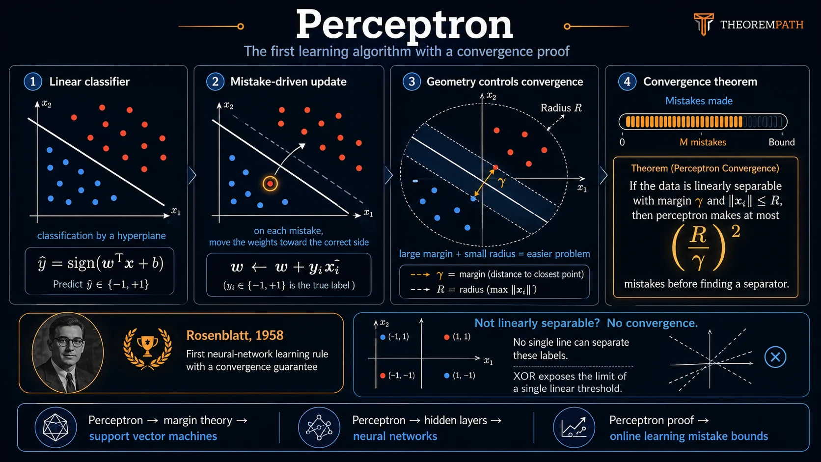
The perceptron is the ancestor of all neural networks. Frank Rosenblatt introduced it in 1958, and it came with something remarkable: a proof that the learning algorithm converges to a correct classifier whenever one exists.

This was the first convergence guarantee for a learning algorithm. The perceptron convergence theorem shows that if the data is linearly separable, the algorithm finds a separating hyperplane in a bounded number of steps. The bound depends only on the geometry of the data (the margin and radius), not on the dimension.

Understanding the perceptron also teaches you what linearity cannot do. The XOR problem, which the perceptron cannot solve, was the catalyst for the "AI winter" and eventually motivated multi-layer networks and backpropagation.

Mental Model

Picture points in $\mathbb{R}^d$ colored red and blue. The perceptron tries to find a hyperplane that separates the two colors. It starts with an arbitrary hyperplane, then adjusts it each time it makes a mistake: nudge the hyperplane toward the misclassified point. If a perfect separating hyperplane exists, this process terminates.

Formal Setup and Notation

We have training data $\{(x_1, y_1), \ldots, (x_n, y_n)\}$ where $x_i \in \mathbb{R}^d$ and $y_i \in \{-1, +1\}$.

Definition

Perceptron Decision Rule

Given a weight vector $w \in \mathbb{R}^d$ and bias $b \in \mathbb{R}$, the perceptron classifies input $x$ as:

$\hat{y} = \text{sign}(w^\top x + b)$

The decision boundary is the hyperplane $\{x : w^\top x + b = 0\}$.

For notational convenience, we absorb the bias into the weight vector by appending a 1 to each input: $x \leftarrow [x; 1]$, $w \leftarrow [w; b]$. The decision rule becomes $\hat{y} = \text{sign}(w^\top x)$.

Definition

Perceptron Learning Rule

Initialize $w^{(0)} = 0$. At each step $t$, pick a training example $(x_i, y_i)$. If it is misclassified ($y_i \cdot w^{(t)\top} x_i \leq 0$), update:

$w^{(t+1)} = w^{(t)} + y_i \, x_i$

If correctly classified, do nothing: $w^{(t+1)} = w^{(t)}$.

The update is intuitive: if $y_i = +1$ and the point is misclassified, we are predicting negative, so we add $x_i$ to $w$ to push the prediction more positive at $x_i$. If $y_i = -1$, we subtract $x_i$.

Core Definitions

Definition

Linear Separability with Margin

A dataset $\{(x_i, y_i)\}$ is linearly separable with margin $\gamma > 0$ if there exists a unit vector $w^*$ ($\|w^*\| = 1$) such that:

$y_i \cdot (w^{*\top} x_i) \geq \gamma \quad \text{for all } i$

The margin $\gamma$ is the minimum distance from any point to the separating hyperplane (after projecting onto $w^*$).

Definition

Radius of the Data

The radius of the dataset is:

$R = \max_i \|x_i\|$

This is the radius of the smallest ball centered at the origin containing all data points.

Main Theorems

Theorem

Perceptron Convergence Theorem

Statement

If the data is linearly separable with margin $\gamma > 0$ and all points have $\|x_i\| \leq R$, then the perceptron algorithm makes at most:

$\left(\frac{R}{\gamma}\right)^2$

mistakes before converging to a linear separator.

Intuition

The bound is purely geometric. The ratio $R/\gamma$ measures how "easy" the classification problem is: large margin and small radius means few mistakes. The bound does not depend on the dimension $d$ or the number of training points $n$. This is remarkable: the perceptron can work in very high dimensions as long as the margin is large relative to the data spread.

Proof Sketch

Track two quantities across the $M$ mistakes made by the algorithm:

Lower bound on $\|w^{(M)}\|$: At each mistake, $w^{(M)} \cdot w^* \geq M\gamma$ (because each update adds at least $\gamma$ to the projection onto $w^*$). Since $\|w^{(M)}\| \geq w^{(M)} \cdot w^*$, we get $\|w^{(M)}\| \geq M\gamma$.

Upper bound on $\|w^{(M)}\|^2$: At each mistake, $\|w^{(t+1)}\|^2 = \|w^{(t)}\|^2 + 2y_i w^{(t)\top} x_i + \|x_i\|^2 \leq \|w^{(t)}\|^2 + R^2$ (the middle term is non-positive because the point was misclassified). So $\|w^{(M)}\|^2 \leq MR^2$.

Combining: $M^2 \gamma^2 \leq \|w^{(M)}\|^2 \leq MR^2$, so $M \leq (R/\gamma)^2$.

Why It Matters

This is one of the earliest and cleanest convergence proofs in machine learning. The potential function argument (tracking both a lower and upper bound on the weight vector) is a proof technique that appears throughout online learning theory. The bound also foreshadows the importance of margin in SVMs.

Failure Mode

If the data is not linearly separable, the perceptron never converges. It cycles through the data making mistakes forever. There is no approximate guarantee. This is the fundamental limitation that motivates soft-margin SVMs and neural networks.

Proof Ideas and Templates Used

The perceptron convergence proof uses a potential function argument: define a quantity (here $\|w^{(t)}\|$) that is bounded from above and below by different functions of the number of mistakes. Squeezing these together gives the bound.

This is the same template used in many online learning proofs, including the analysis of the Winnow algorithm and online mirror descent.

Canonical Examples

Example

Perceptron on 2D data

Consider four points: $(1,1)$ with label $+1$, $(2,1)$ with label $+1$, $(-1,-1)$ with label $-1$, $(-1,0)$ with label $-1$. These are linearly separable. The perceptron starts at $w = (0,0)$, encounters $(1,1)$ and misclassifies it (predicts 0), updates to $w = (1,1)$. The next point $(-1,-1)$ is correctly classified ($w^\top x = -2 < 0$, predict $-1$). After a few passes, the algorithm converges.

Common Confusions

Watch Out

The perceptron finds a separator, not the best separator

The perceptron finds some separating hyperplane, not the maximum-margin one. The specific hyperplane depends on the order in which points are processed and the initialization. Finding the maximum-margin hyperplane is the job of support vector machines.

Watch Out

The XOR problem is about representational capacity, not the algorithm

The perceptron cannot solve XOR because no single hyperplane can separate the four XOR points. This is a limitation of the linear model, not of the learning algorithm. Adding a hidden layer (multi-layer perceptron) solves XOR, but the perceptron convergence theorem no longer applies to the training of multi-layer networks.

Summary

• Decision rule: $\hat{y} = \text{sign}(w^\top x + b)$
• Update on mistake: $w \leftarrow w + y_i x_i$
• Convergence bound: at most $(R/\gamma)^2$ mistakes if data is linearly separable with margin $\gamma$
• The bound depends on geometry (margin and radius), not dimension
• Does not converge if data is not linearly separable
• Historically: the first learning algorithm with a convergence proof (1958)

Exercises

ExerciseCore

Problem

The perceptron is run on a dataset where $R = 10$ and the margin is $\gamma = 0.5$. What is the maximum number of mistakes the algorithm can make?

Hint

Reveal Solution

ExerciseCore

Problem

Show that the XOR function (inputs $(0,0), (0,1), (1,0), (1,1)$ with labels $-1, +1, +1, -1$) is not linearly separable. Why does this kill the perceptron?

Hint

Reveal Solution

ExerciseAdvanced

Problem

Prove that the perceptron convergence bound $(R/\gamma)^2$ is tight: construct a dataset in $\mathbb{R}^d$ where the perceptron makes exactly $(R/\gamma)^2$ mistakes.

Hint

Reveal Solution

References

Canonical:

• Rosenblatt, "The perceptron: a probabilistic model for information storage and organization in the brain" (1958)
• Novikoff, "On convergence proofs for perceptrons" (1962)

Current:

• Shalev-Shwartz & Ben-David, Understanding Machine Learning (2014), Chapter 9

• Mohri, Rostamizadeh, Talwalkar, Foundations of Machine Learning (2018), Chapter 8

• Hastie, Tibshirani, Friedman, The Elements of Statistical Learning (2009), Chapters 3-15

• Bishop, Pattern Recognition and Machine Learning (2006), Chapters 1-14

Next Topics

The natural next steps from the perceptron:

• Support vector machines: finding the maximum-margin separator
• Feedforward networks and backpropagation: overcoming the linear separability limitation