Knowledge Distillation

Why This Matters

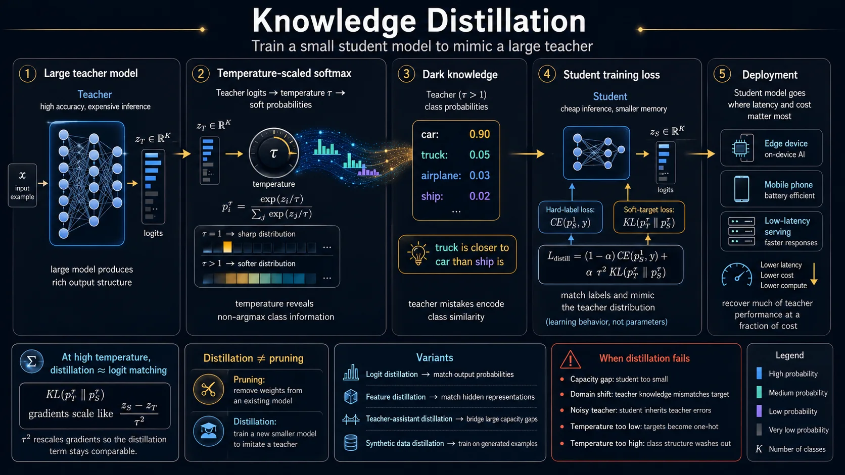
Large models (billions of parameters) achieve strong performance but are expensive to serve. A 175B parameter model requires multiple GPUs for inference, making it impractical for edge and on-device ML deployment. Knowledge distillation trains a small "student" model to approximate a large "teacher" model, often recovering most of the teacher's accuracy at a fraction of the cost.

Distillation is not just compression. The student trained on teacher outputs often outperforms an identical architecture trained only on hard labels. The teacher's soft probability distribution over classes contains information that hard labels discard.

Formal Setup

Let $f_T$ be a teacher network and $f_S$ a student network. Both map inputs $x$ to logit vectors $z \in \mathbb{R}^K$ for $K$ classes.

Definition

Temperature-Scaled Softmax

For logits $z = (z_1, \ldots, z_K)$ and temperature $\tau > 0$:

$p_i^\tau = \frac{\exp(z_i / \tau)}{\sum_{j=1}^K \exp(z_j / \tau)}$

At $\tau = 1$, this is the standard softmax. As $\tau \to \infty$, the distribution approaches uniform. As $\tau \to 0$, it approaches a one-hot vector at the argmax.

Definition

Distillation Loss

The distillation loss combines two terms:

$\mathcal{L}_{\text{distill}} = (1-\alpha) \cdot \mathcal{L}_{\text{CE}}(p_S^1, y) + \alpha \cdot \tau^2 \cdot \mathrm{KL}(p_T^\tau \| p_S^\tau)$

where $p_T^\tau$ and $p_S^\tau$ are the teacher and student softmax outputs at temperature $\tau$, $y$ is the hard label, $\mathrm{KL}$ is the KL divergence, and $\alpha \in [0,1]$ balances the two terms. The $\tau^2$ factor compensates for the reduced gradient magnitudes at high temperature.

Why Soft Targets Help: Dark Knowledge

Consider a teacher trained on CIFAR-10. For an image of a car, the teacher might output: car 0.9, truck 0.05, airplane 0.03, ship 0.02. The hard label says only "car." But the teacher's soft distribution encodes that trucks look more like cars than airplanes do, and airplanes look more like cars than ships do.

This relational information between classes is what Hinton et al. (2015) call dark knowledge. It is invisible in the hard labels but present in the teacher's soft outputs. High temperature amplifies these small probabilities, making the dark knowledge more accessible to the student.

Proposition

Distillation Gradient at High Temperature

Statement

At high temperature $\tau \gg |z_i|$ for all logits, the gradient of the KL divergence term with respect to the student logits $z_S$ approximates:

$\frac{\partial}{\partial z_{S,i}} \mathrm{KL}(p_T^\tau \| p_S^\tau) \approx \frac{1}{K\tau^2}(z_{S,i} - z_{T,i})$

That is, the distillation loss encourages the student logits to match the teacher logits, weighted by $1/\tau^2$. The $\tau^2$ prefactor in the distillation loss cancels this, giving gradients of order $1/K$.

Intuition

At high temperature, softmax becomes nearly linear: $p_i^\tau \approx 1/K + z_i/(K\tau)$. The KL divergence between two nearly-uniform distributions reduces to a squared difference between the logit vectors. Distillation at high temperature is approximately matching teacher logits, which is a regression problem. This is gentler than matching sharp distributions and provides richer gradient signal.

Proof Sketch

Taylor expand $\exp(z_i/\tau)$ around $z_i = 0$ for large $\tau$: $\exp(z_i/\tau) \approx 1 + z_i/\tau + z_i^2/(2\tau^2)$. The softmax becomes $p_i^\tau \approx 1/K + z_i/(K\tau) - \bar{z}/(K\tau)$ where $\bar{z}$ is the mean logit. Substitute into the KL formula and differentiate.

Why It Matters

This explains the $\tau^2$ factor in the loss and why moderate temperatures ($\tau \in [2, 20]$) work best. Too low: the student just sees near-one-hot targets. Too high: all class information is washed out. The sweet spot preserves the ranking and relative magnitudes of teacher logits.

Failure Mode

The high-temperature approximation breaks when some logits are much larger than $\tau$. For confident teacher predictions (one logit dominating), the soft distribution is still nearly one-hot even at moderate $\tau$, and the student recovers little dark knowledge for that example.

Logit Distillation vs. Feature Distillation

Logit distillation (Hinton et al., 2015) matches the teacher's output distribution. This is the standard approach described above.

Feature distillation (Romero et al., 2015, "FitNets") matches intermediate representations. The student is trained so that its hidden layers approximate the teacher's hidden layers. This requires choosing which layers to align (often the middle layer) and a projection to handle dimension mismatches.

Feature distillation can be combined with logit distillation. The advantage: it provides more supervision signal, especially when the student architecture is very different from the teacher. The disadvantage: choosing which layers to align and how to project between them introduces design choices with no clear optimal answer.

When Distillation Fails

Distillation does not always improve over training from scratch.

Capacity gap. If the student is too small to represent the teacher's function, distillation cannot help. The student will learn a biased approximation. Mirzadeh et al. (2020) showed that extremely large teacher-student gaps can actually hurt, and proposed "teacher assistant" distillation (distill teacher to medium model, then medium model to small model).

Task mismatch. If the teacher was trained on a different distribution than the student's target, the soft labels may be misleading. Domain shift between teacher training data and student deployment data degrades distillation.

Label noise. A teacher trained on noisy labels will produce soft targets that encode noise patterns. The student faithfully learns these errors.

Common Confusions

Watch Out

Distillation is not the same as model pruning

Pruning removes weights from an existing model. Distillation trains a new (smaller) model to mimic a larger one. The student architecture can be completely different from the teacher. Pruning preserves the architecture but makes it sparse; distillation allows architectural changes.

Watch Out

The tau-squared factor is not optional

Without the $\tau^2$ scaling in the loss, the gradients from the KL term shrink as $1/\tau^2$ when temperature increases. The $\tau^2$ factor compensates for this, ensuring the distillation gradient remains at a useful magnitude regardless of temperature.

Canonical Examples

Example

MNIST teacher-student

Teacher: 3-layer MLP with 1200 hidden units per layer (3.6M parameters, 1.2% test error). Student: 2-layer MLP with 800 hidden units (0.96M parameters). Trained on hard labels: 1.9% test error. Trained with distillation ($\tau = 8$, $\alpha = 0.7$): 1.4% test error. The distilled student, with 3.7x fewer parameters, nearly matches the teacher and cuts the test error from 1.9% to 1.4% compared with training from scratch.

Exercises

ExerciseCore

Problem

For a 3-class problem with teacher logits $z_T = (5, 3, 1)$, compute the teacher's softmax output at $\tau = 1$ and $\tau = 5$. Which temperature reveals more about the relationship between classes 2 and 3?

Hint

Reveal Solution

ExerciseAdvanced

Problem

Show that when $\tau \to \infty$, the KL divergence $\mathrm{KL}(p_T^\tau \| p_S^\tau)$ approaches a scaled squared Euclidean distance between the logit vectors (after centering). What is the scaling factor?

Hint

Reveal Solution

References

Canonical:

• Hinton, Vinyals, Dean, "Distilling the Knowledge in a Neural Network" (2015), Sections 1-3
• Romero et al., "FitNets: Hints for Thin Deep Nets" (ICLR 2015)

Current:

• Gou et al., "Knowledge Distillation: A Survey" (IJCV 2021), Sections 2-4
• Mirzadeh et al., "Improved Knowledge Distillation via Teacher Assistant" (AAAI 2020)

Next Topics

Distillation connects to model compression, deployment optimization, and the broader question of what knowledge neural networks actually learn.